CS 184: Computer Graphics and Imaging, Spring 2019
Project 1: Rasterizer
Beverly Pan
Section I: Rasterization
Part 1: Rasterizing single-color triangles
To rasterize a triangle, I first implemented a function that fills a pixel's sub-pixels with a specified color. Once this function was implemented, I began the real meat of the work: implementing the sampling.
For basic rasterization, where sample rate = 1, I first set up two for loops that iterate from the min to max triangle x value and the min to max triangle y value. Next, I set up a function to calculate line equations. I used this to set up a point-in-triangle test, which uses three line tests. At each point I iterate through, I check if the point at (x+.5, y+.5) is inside the triangle - that is, if lineEQ(x+.5, y+.5) >= 0 for all points that make up the triangle. Here, adding +.5 to x and y is simply convention for finding the center of the sample. Technically, we should check if lineEQ is strictly greater than 0; but, for the purposes of this assignment, we can also consider a point on the line to be inside the triangle.
However, the three line tests are not complete yet. Our triangle vertices are not necessarily given in a counterclockwise order. To account for points given in a clockwise order, we should also check if lineEQ(x+.5, y+.5) < 0 for all points that make up the triangle.
Once a location passes the point-in-triangle test, we need to fill the samplebuffer's pixel (x, y) with the input color.
The algorithm I implemented does no worse than one check of each sample within the bounding box of the triangle. In fact, it performs exactly one check of each sample within the bounding box, since I perform the point-in-triangle test at each point in my for loops.
Part 2: Antialiasing triangles
To implement supersampling, I modified my basic rasterization code to account for sample size > 1. In this case, I iterated through two more for loops both with lower bound = 0 and upper bound < sqrt(sample_rate). This lets me sample NxN, or sample_rate, times within each screen sample, where N = sqrt(sample_rate).
Now, instead of offsetting x and y by .5, we have to more explicitly calculate each offset to find the center of each supersampled pixel. I calculated this to be 1/(sqrt(sample_rate) * 2). Next, to find the x and y border values in each of the supersampled pixel, we add (Nw*offset) or (Nh*offset), where Nw and Nw refer to the current indexes of the supersampling for loops. All together, I use the points (x + offset + (Nw*offset), y + offset + (Nh*offset)) to calulate the three line equations.
Now, instead of filling the current pixel with the input color (which negates the work done by supersampling), we fill each subpixel directly with the input color. Next, I implement a function that will average the subpixel colors when to use as the output color.
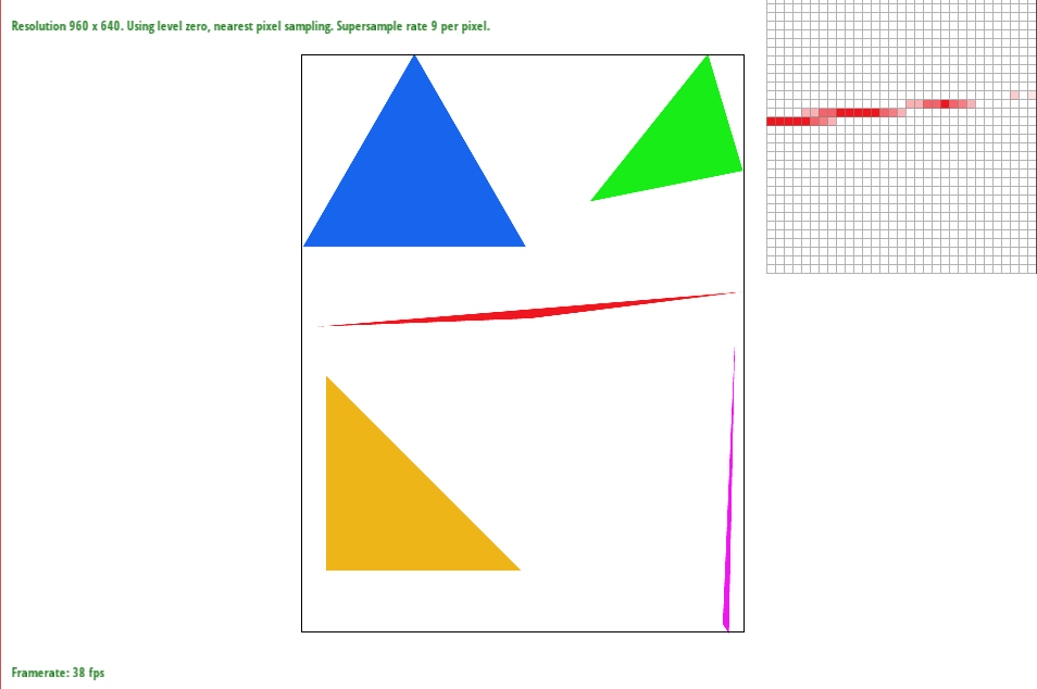
Supersampling is useful because it allows us to avoid aliasing artifacts such as the "jaggies" mentioned in Part 1. Supersampling is method we can use to anti-alias. To supersample, we calculate and use gradient colors, which can be thought of as removing high-frequency changes in color.
In the above images, we can see how supersampling reduces the jaggies effect. Where using sample rate = 1 gives sharp edges and draws strange disconnected triangle edges, sample rate = 16 gives much smoother-looking edges and seems to connect the triangle edges back to the main triangle body.
The downside to supersampling as an antialiasing method is the much increased number of calculations needed.
Part 3: Transforms
To make a DabBot out of a basic cubeman, I used many rotate and a few translate transforms. I tilted cubeman's head to face forward into his elbow and translated it a bit towards the screen's left to compensate for the fact that the rotate is centered around the middle of the box (as opposed to bottom of his head, where a neck would be). To make his leg bent, I rotated his entire leg forward, then rotated just his shin back, taking into consideration that cubeman is made with a hierarchal structure. I made DabBot's dab in a similar method.
Section II: Sampling
Part 4: Barycentric coordinates
Barycentric coordinates are a coordinate system that allows us to interpolate across a triangle. They interpolate values at the vertices - the values can be anything from color (as in the image above), to texture coordinates, positions, normal vectors, etc.
To calculate the barycentric coordinates, we first calculate coordinate "weights" alpha, beta, and gamma. Alpha, beta, and gamma are constrained by the equation: alpha + beta + gamma = 1. We can calculate alpha using the line equations: lineEQbc(x, y)/lineEQbc(xA, yA). "bc" refers to the points on the triangle that are not weighted by alpha; (xA, yA) refers to the point on the triangle that is weighted by alpha. Beta can be calculated in the same way, and gamma can be calculated with the constraint in mind as 1 - alpha - beta.
After calculating alpha, beta, and gamma, we can calculate the barycentric coordinates (x, y) = alpha * A + beta * B + gamma * C.
Part 5: "Pixel sampling" for texture mapping
To implement pixel sampling for texture mapping, I first computed the computed the appropriate (u, v) coordinate (using barycentric coordinates). Next, based on the appropriate input for how to sample (using nearest pixel sampling or bilinear sampling), I implemented actual sampling methdos:
Nearest pixel sampling takes the nearest pixel to the point of interest for information. I implemented this by calculating the distance between the current sampling point and the four surrounding pixels, finding the pixel with the minimum distance, and taking the relevant information (in this case, color) from that pixel.
On the other hand, bilinear filtering takes the four nearest pixels and linearly interpolates, or LERPs, through them. To implement this, I performed two LERPS in the horizontal direction and a final LERP in the vertical direction. Because bilinear filtering interpolates, it will generally give a better output than nearest pixel sampling.
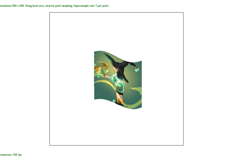
In the images above, we can see how bilinear sampling produces a better image (smoother looking lines) than nearest pixel sampling. In general, bilinear sampling will be much better than nearest pixel sampling when the source image has low resolution, since nearest pixel sampling will not produce enough information. However, when the resolution is high, nearest pixel sampling is similar to bilinear sampling because there is more information to pick from.
Part 6: "Level sampling" with mipmaps for texture mapping
Level sampling allows us to adjust our texture for the case when textures are minified. In this case, the texture is downsampled and stored. These are called mipmaps. We want to choose the level of the mipmap whose resolution best approximates the screen sampling rate.
To implement this functionality, I first calculate the correct mipmap level, D, using D = log2(L), where L is the max of sqrt((du/dx)^2 + (dv/dx)^2) or sqrt((du/dy)^2 + (dv/dy)^2). This required finding barycentric coordinates of (x+1, y) and (x, y+1) (done in the rasterize function). Next, I calculated the (du/dx, dv/dx) and (du/dy, dv/dy) values and scaled them by the width and height of the texture image, respectively. Finally, I used the equation listed above to find D.
Using mipmaps requires more storage to store the downsized texture information. However, the higher the level, the less storage is required for the mipmap. It also decreases the render time and reduces aliasing.
Supersampling is good for antialiasing, since it allows us to pick up and average more information from the source, but scales badly precisely because of this. On the other hand, bilinear sampling is much faster and gives similarly high-quality results - linear interpolation gives pretty good information since it can be thought of as taking a weighted average.


