
CS 184: Computer Graphics and Imaging, Spring 2019
Project 3-1: PathTracer
Beverly Pan


Overview
In this project, I implemented a renderer that uses a pathtracing algorithm to render scenes with physical lighting. I began with simple functions that generate rays and check for ray-object primitive intersections, then implemented a bounding volume hierarchy to accelerate and optimize ray-surface intersections processing. With this implemented, scenes containing geometry with hundreds of thousands of triangles rendered incredibly quickly (< 5 seconds!) whereas before, such scenes would take minutes to render (if they rendered, at all). Next, I implemented lighting calculations in the scene, including direct illumination (including hemisphere and importance sampling) and global illumination. This implementation used Monte Carlo integration to estimate the direct lighting. After completing this step, I was able to render beautiful scenes with direct and indirect lighting. Finally, I implemented adaptive sampling, which tries to optimize the samples taken per pixel by checking if the pixel has already converged, and terminating sampling for a pixel if it has.
After completing this project, I am much better able to understand how path tracing works and methods for optimizing it without sacrificing (too much of) the resolution of the final image.
Part 1: Ray Generation and Intersection
To make a physically-based renderer, we begin with the physically-based model of light which suggests light travels in straight lines from light sources to the eye. This means we can implement lighting as light rays which travel from light sources/bounce off objects in our scene to the camera. However, light an hit a surface and bounce off in any direction, which means most of the light rays coming from an object or light source do not ever reach the camera - which is incredibly inefficient. So, we can instead use camera rays, creating images by casting rays for each pixel of our final image and checking them against light sources for shadows.
I implemented camera rays by simpling writing a function that transforms an input to my camera-space coordinate system, then creating a Ray object which takes in an origin position and direction in world space coordinates. We can then implement a recursive ray tracing algorithm for multiple light bounces, which is realistic; I implemented this in later parts of this project.
Next, it is important to check for ray-surface intersections. These intersections can determine if the ray we are tracing has hit an object; if the object we have hit is directly illuminated by the light source; if an object is occluded by another object; etc. I implemented the Moller Trumbore algorithm to test for triangle intersection.
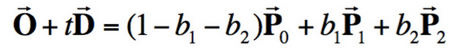
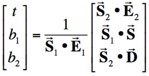
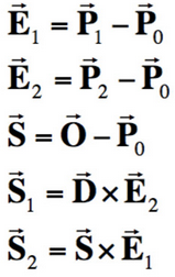
We can obtain result vector [t, b1, b2]T, where t is the time of intersection and (1-b1-b2, b1, b2) are barycentric coordinates that describe the intersected point in triangle with vertices P0, P1, and P2. This algorithm finds t, b1, and b2 that solves the equation we obtain by setting the ray equation, O + tD, equal to the point on the triangle we are intersecting, (1-b1-b2)P0 + b1P1 + b2P2. In my implementation, I calculate t, b1, and b2 using this algorithm. If t occurs between my ray's minimum and maximum possible times (which are originally set as the camera's clipping planes) and the barycentric coordinates (1-b1-b2), b1, and b2 are valid (they are between 0 and 1), then an intersection has occurred and I store information about t, the surface normal at the intersection, what kind of primitive I have hit (a triangle), and the bsdf in an Intersection variable.

After implementing this, I was able to render just the walls of the CBspheres_lambertian file. To see the spheres, I implemented a sphere intersection check, which determines whether there are 0, 1, or 2 intersection times between my ray and a sphere using the quadratic formula.
Part 2: Bounding Volume Hierarchy
After completing Part 1, I could render very simple scenes; however, rendering slightly more complex scenes or scenes containing meshes with more triangles was incredibly slow. This is because the simple implementation was checking every ray against every object, even if the ray completely missed the object! To speed up the rendering process, we can use the idea of axis-aligned bounding volumes and object partitions, or a bounding volume hierarchy. (Basically, make a tree. Trees are good for the environment. And optimization.)
First, I constructed a BVH. In a BVH, each internal node stores a bounding box of all the objects inside it and references to children nodes. Each leaf node stores a list of object primitives and their aggregate bounding box. In my implementation, I first create a bounding box for each node. I check if the node is a leaf - which is true if the size of the input list of primitives is <= max_leaf_size, where max_leaf_size is a somewhat arbitrary cap on the max number of primitives we can have in a leaf. If the node is not a leaf, I split my primitives (using the axis of the bounding box's largest dimension, which I'll call [axis]) based on a somewhat arbitrarily-chosen heuristic, the average of all the primitives' centroids. The primitives are sorted into a left or right child based on if their centroid's [axis] value is less than or greater than the average-centroid-bbox's [axis] value.


The above is a visual representation of my BVH on cow.dae. My BHV splits primitives based on the coordinates of the average centroid of all the primitives left to sort.
Next, I implemented a recursive BVH intersection algorithm that not only returns true if there exists an intersection, but also stores information about the closest of all intersections in an Intersection variable. To do so, I use a "hit" boolean to keep track of whether or not there has been an intersection. An automatic-return case (returning false) occurs if my ray does not intersect the current node's bounding box at all. If my current node is a leaf, then I can iterate through all the primitives in the node and check their intersections. Because earlier I wrote my primitive intersection methods to also update an inputted Intersection variable with the min intersection time, the intersection check itself will actually ensure I keep the closest Intersection information. Finally, if my current node is not a leaf, I recursively call this BVH intersection function on the node's left and right children.


After implementing the BVH, I was able to render much more complex scenes/geometry at a much higher speed. For example, before BVH, the cow.dae file took 2min 26s (146s) to render. With BVH implemented, the file rendered in about 2s. The maxplanck.dae and CBlucy.dae files would not even render on my laptop without BVH; with BVH, they both rendered in 4 to 6 seconds. (It was interesting to note that with BVH, opening maxplanck.dae and CBlucy.dae actually took more time than rendering them). By checking for bounding box intersections before checking primitive intersections, we can quickly "throw away" nodes with bounding boxes/primitives that are never intersected. With a good heuristic and/or a heuristic that is good for the particular scene we are rendering, we can effectively reduce our runtime from linear Θ(n) to logarithmic Θ(log(n)) (n is the number of primitives in the scene).
Part 3: Direct Illumination
In this part, I implemented two direct lighting estimation methods: one sampling uniformly in a hemisphere around each intersection, and another using importance sampling. The estimation of the resulting irradiance was done using concepts from Monte Carlo Integration.

To implement uniform sampling across a hemisphere, I first calculated the probability density function (pdf) (1 / (2*π)). Next, for num_samples of samples, I obtain a vector sample of the unit hemisphere, and convert it into world coordinates. I create a ray, using this sample as the ray's direction and adding it to hit_p, my hit point, for the ray's origin. If this ray intersects my BVH (I use my BVH intersect method from Part 2, so checking for an intersection will also populate an Intersection variable, if one exists), I can get the material's emitted light. The emitted light I obtain is an incoming radiance; to transform it into irradiance, I multiply by the BSDF and a cosine term. To get the Monte Carlo Estimate, I also divide this result by the pdf, and finally, I return the accumulated result from all my samples, averaged.

Unlike hemisphere sampling, importance sampling samples every light source in the scene. To implement this, I begin by looping over all the lights in the scene. If the current light is a delta light, I only sample once since all samples are the same; otherwise, I sample as many times as specified. My sampling method returns the incoming radiance, as well as the pdf, a probabilistically sampled direction vector (from the hit point to the light), and the distance from the hit point to the light, by pointer. After converting the direction vector from world to object space, I check that its z coordinate is positive (i.e., the light is in front of the object and will give a result visible to us). Next, I cast a shadow ray from the hit point to the light check whether it is occluded by other objects/surfaces. If there is no intersection between my BVH and this ray, then I can safely accumulate the irradiance at this hit point (performing the same calculation as in hemisphere sampling, including multiplying the irradiance sample we obtained by the BSDF and a cosine term, then dividing by pdf). Finally, I divide the accumulated samples for each light by the number of samples I took, then return the accumulated results of every light in the scene.


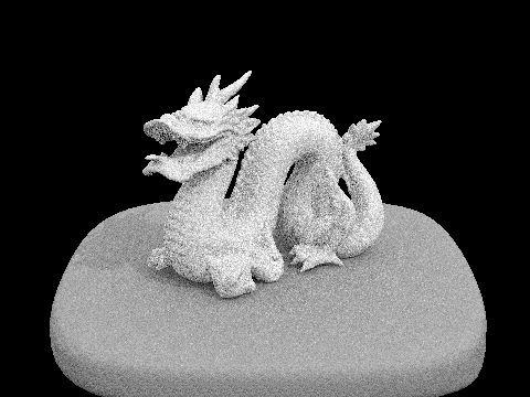

The above renders are taken of dragon.dae, using light sampling
In these dragon.dae renders, I test light sampling using 1 sample and increasing numbers of light rays. With fewer light rays, there is a lot of noise in the soft shadows (as well as overall picture). At about 16 light rays, we can begin to properly see the difference between the darker shadow right underneath the dragon and the lighter, longer shadows cast to the side. As we can see, more samples = more information; to get enough information for this dragon scene to look "good", we should probably use even more light rays, or increase the number of samples we take (one is not very much).


The above renders are taken of CBbunny.dae, both rendered at 64 samples, 32 light rays
Here, we see that uniform hemisphere sampling and light/importance sampling produces very different results with the same amount of samples + light rays. Uniform hemisphere sampling is much granier (more noise) because we take samples in all directions around a point. So, we sample only some rays that actually point towards a light; incoming radiance is zero for most directions in this bunny scene and we get many dark spots. On the other hand, importance sampling prioritizes those samples that will actually contribute more to the result. By integrating over and sampling from only the lights, can ensure that all our samples will be taken from angles where incoming radiance could be non-zero. Thus, we can achieve a much smoother, less noisy image.
Part 4: Global Illumination


In this part, I implemented global illumination. While direct lighting produces some nice images, it only accounts for one bounce of light - which is not very realistic. In real life, light bounces multiple times off surfaces, letting areas where light does not directly hit still be illuminated.
To implement global illumination, I first created a method that returns the radiance at zero bounces of light - that is, the light emitted from a light source the directly travels towards the camera. Next, I implemented a method that returns the radiance at one bounce of light. This method simply returns the direct lighting methods I created in Part 3: hemisphere sampling if requested, or importance sampling otherwise.
Next, I implemented the recursive method that accounts for at least one bounce of light. This method also uses Russian Roulette to randomly (and unbiasedly) terminate sampling, to decrease the amount of render computations necessary for the scene. In this method, I begin by setting a vector L_out (which I use to accumulate my radiances) to the result from one bounce. Next, I check that my max ray depth is greater than one (otherwise, return immediately), my pdf is greater than 0 (if pdf = 0, I might eventually divide by 0 which results in Unsavory White Specks), and that the new ray I am about to shoot from the current point intersects my BVH (if there is nothing to hit, I should stop trying). If I pass these conditions, I then check if the current ray's depth is the same as the max ray depth. If this is the case, that means I am on the first bounce and should guarentee that there is another bounce. So, I should accumulate L_out with a recursive call to this method, scaling the resulting radiance (like before) by the BSDF and a cosine factor, then dividing by the pdf. In this recursive call, I use the new ray I created earlier, which has a depth value that is decremented from the current ray's value. That way, I will eventually be able to terminate the recursion even without Russian Roulette because the ray depth will no longer be >1.
If my current ray is less than the max ray depth, I can use Russian Roulette to randomly terminate the ray. To do this, I call a coin_flip method and use a termination probability of 0.3 (the same as a continuation probability of 0.7). Should Russian Roulette tell me to continue sampling, I then check that the current ray's depth is greater than 1. If this condition is also true, I can accumulate L_out with a recursive call to this method, again using the new ray created earlier. I also scale the resulting radiance by BSDF and a cosine factor, then divide by the pdf, as before. However, I also divide by (1 - termination probability) (that is, the continuation probabiity, or 0.7) because I used Russian Roulette.
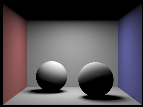

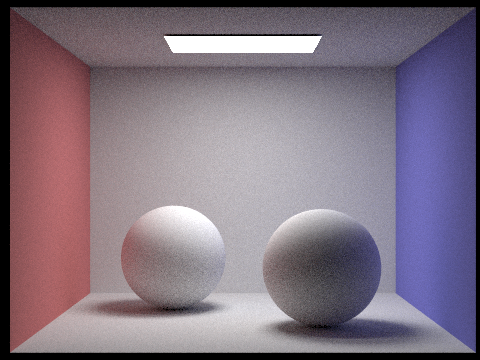
The above are renders of CBspheres_lambertian.dae, taken with 4 light rays and maximum ray depth 5


The above renders are of CBbunny.dae, taken with 1024 samples and 4 light rays.
In the images of CBbunny.dae above, we can see that increasing the max ray depth increases the amount of light in the scene. We begin with 0 bounces, where we can only see the emitted light from the light source. At one bounce, we get almost the same image as we did in Part 3 using only direct lighting + importance sampling - the difference being the emitted light visible at the top. With increased max ray depth, we get a lighter and lighter image and more colored light hitting uncolored surfaces. Importantly, because of our probabilistic random termination, the render time for these images at high max ray depth was not incredibly much longer than images at lower max ray depths. Especially in the case of max ray depth of 100, it is incredibly unlikely that we recurse all 99 times in our at-least-one-bounce method (the probability of that happening in my implementation is (0.7)99, which is a Very Small Number).


The above are renders of CBspheres_lambertian.dae, taken with 4 light rays and max ray depth 5
In the comparisons of CBspheres_lambertian.dae above, we can see clearly that increasing sample size decreases the noise of the render.
Part 5: Adaptive Sampling
After completing Part 4, I was able to render beautiful images using global illumination; however, we can still optimize our rendering further by using adaptive sampling. Adaptive sampling changes the sample rate based on how quickly a pixel converges. Some pixels converge quickly, so we should take fewer samples if possible; other pixels require many samples to reduce noise, so we should use as many samples as possible (up to our specified max).
To implement adaptive sampling, I updated the raytrace_pixel(x, y) method (x and y are the inputs specifying which pixel we are raytracing for) with a simple algorithm. In each pixel, we want to sample ns_aa times (ns_aa being our specified total samples). Every 32 samples, I check if the pixel has converged by checking if:
I <= maxTolerance * μ
where I = 1.96 * σ / sqrt(n), maxTolerance is 0.05 by default, and μ is the mean. We calculate the mean and standard deviation as such:
| σ = s1 / n | μ = (1 / (n - 1)) * (s2 - (s12 / n)) |
where
| s1 = ∑k=1n xk | s2 = ∑k=1n xk2 |
where xk is the illuminance at each sample k.
If the pixel has converged, I update our sampleCountBuffer (which stores the number of samples taken at each pixel). Updating the sampleCountBuffer enables us to create sample rate images that indicate how many samples we are taking at each pixel using red colors to indicate high sampling rates, and blue to indicate low sampling rates.


The above renders are of CBbunny.dae, taken with 2048 samples, 1 light ray, max ray depth 5.
In the sample rate image, red represents high sampling rates; blue represents low sampling rates.